Plume pattern - Hail Creek 15^th September 2019 - Orbit 09956

For detailed investigation, we selected orbit 09956, which is used in insert (f) of Figure 1 of Sadavarte, et al., 2021 .

Mean Sea Level Pressure

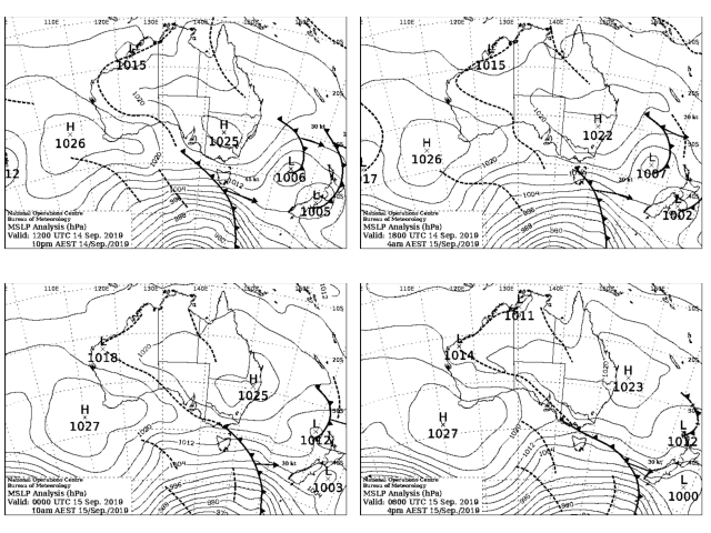
The initial set of 6-hourly MSLP charts from 14 September 2024 00Z to 15 September 2024 06Z was downloaded from the Bureau of Meteorology's chart archive BoM Chart Archive 2025 (See Figure 25). The charts show a slow moving high pressure system centred over northern New South Wales dominating the flow over the study area. Notably, the pressure gradient is very weak, indicating light winds. A secondary feature of interest is a weak trough extending from the Gulf of Carpentaria southward. This configuration is climatologically consistent with the typical winter position of the STR over Australia, extending from a high pressure system west of Perth across the continent toward a high moving eastward from northern New South Wales into the Pacific Ocean. The conditions depicted in these charts are favourable for the formation of a stable nocturnal boundary layer SNBL.

Moranbah AWS

Observations from the Moranbah AWS indicate clear conditions with no cloud or precipitation, and visibility greater than 10 ($\mathrm{km}$) (this information is omitted from the Table 19 for simplicity). The data show two warm winter days with maximum temperatures reaching 30 ($°C$), followed by a cool night driven by strong radiative cooling. The temperature dropped from a daytime maximum of 30.6 ($°C$) at 05:30 Z on 14 September 2019 to a minimum of 7.5 ($°C$) before sunrise at 20:00 Z the same day. Winds overnight were very light, with an extended period of calm conditions until around 22:00 Z, after which an initially weak northerly flow shifted to easterly, reaching 22.3 ($\frac{\mathrm{km}}{\mathrm{hour}}$) by 04:00 Z on 15 September 2019. Note that when the 10-minute average wind speed falls below 1.8 ($\frac{\mathrm{km}}{\mathrm{hour}}$), the AWS reports both wind speed and direction as zero.

The estimated sunset at Hail Creek on 14 September 2019 was 08:02 Z, and sunrise occurred at 20:05 Z Australian Government, Geoscience Australia, Sunrise, Sunset & Twilight Times. . Based on the AWS observations, the site entered the Stable Nocturnal Boundary Layer (SNBL) at approximately 11 Z (around three hours after sunset) and transitioned back into the Convective Mixed Layer (CML) at about 22 Z, roughly two hours after sunrise.

TROPOMI

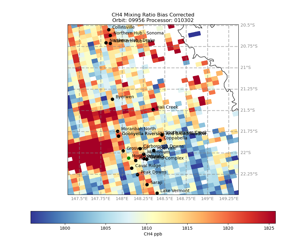
The data retrieved for orbit 09956 are shown in Figure 26. Some striping is visible in the image. Although the orbit meets all domain quality filters, it fails the albedo SWIR orbit filter. However, because this orbit was used in the original study, we include it in this discussion (image adjustments in the original analysis may have mitigated this issue).

Within the domain defined by Sadavarte, et al., 2021 , the TROPOMI dataset contains 2,033 pixels with qa = 1. The correlation coefficients within this domain are:

• albedo SWIR: 0.092
• albedo NIR: 0.010
• aerosol SWIR: 0.106
• aerosol NIR: 0.110

At the orbit level, however, the following values fail the required thresholds:

• albedo SWIR: 0.514
• albedo NIR: 0.274
• aerosol SWIR: 0.324
• aerosol NIR: 0.343

In the TROPOMI image, two major plumes extend westward: one originating from the Hail Creek mine and another, larger plume from the Bowen Basin mines near the Moranbah North marker. Elevated ${\mathrm{CH}}_4$ concentrations are also evident east of Hail Creek along the Pacific coast. As expected, many pixels between the mine region and the coast are missing due to terrain effects over the ranges.

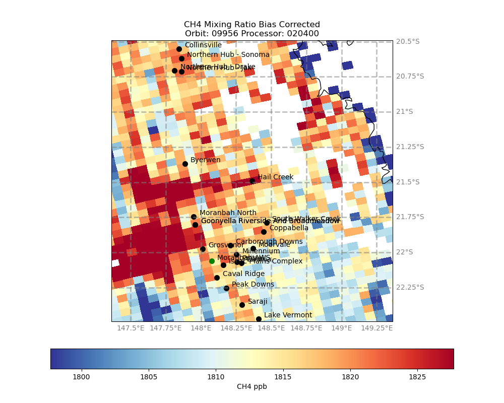
Two versions of this orbit are available from the Copernicus Data Store. The version generated with processor 010302, created on 21 September 2019, was likely the one used in the original paper. A later version, processed with 020400 on 14 November 2022 and shown in Figure 27, exhibits several differences.

When comparing the two products, the processor 020400 output shows ${\mathrm{CH}}_4$ values approximately 5 ($\mathrm{ppb}$) higher. In addition, more pixels are flagged as valid, particularly east of Hail Creek over the mountain ranges and near the Pacific coast.

HYSPLIT

We ran forward HYSPLIT simulations in trajectory mode for puffs released at Hail Creek at hourly intervals from 2019-09-14 04Z (approximately 2p.m. local time and the time of the previous TROPOMI overpass) through 2019-09-15 03Z. Each puff was released at the midpoint of the boundary layer. The simulations used the GFS meteorological dataset at 0.25° resolution, referred to as GFSQ in the HYSPLIT interface.

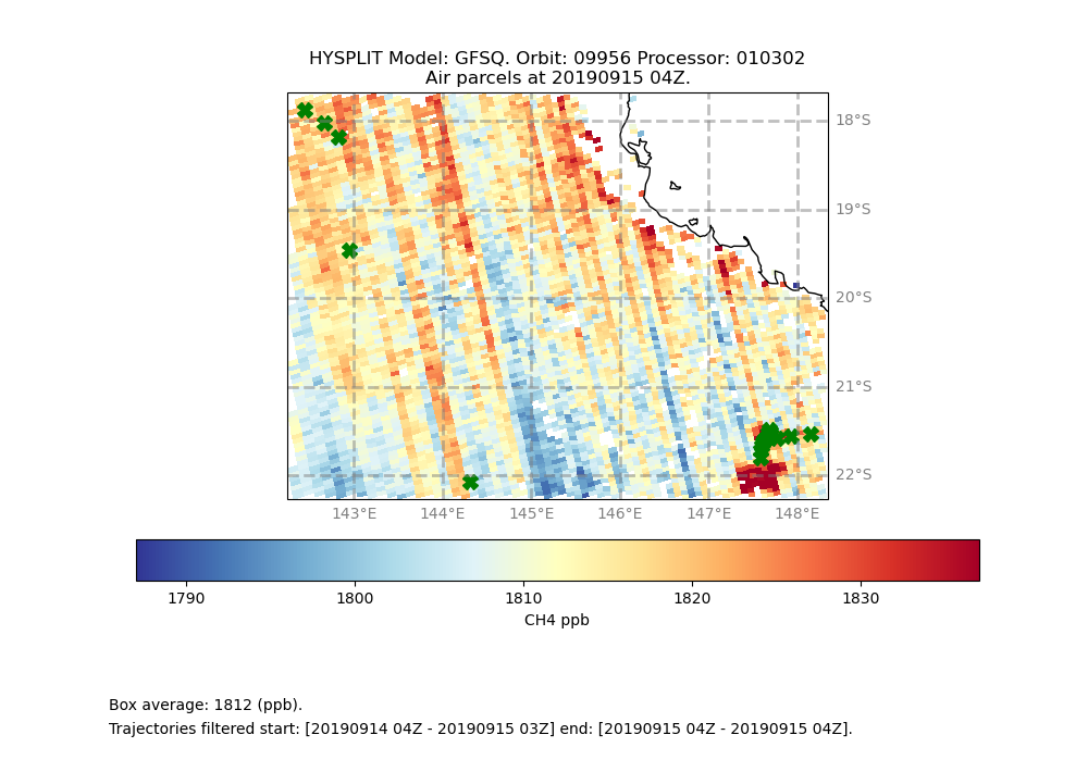
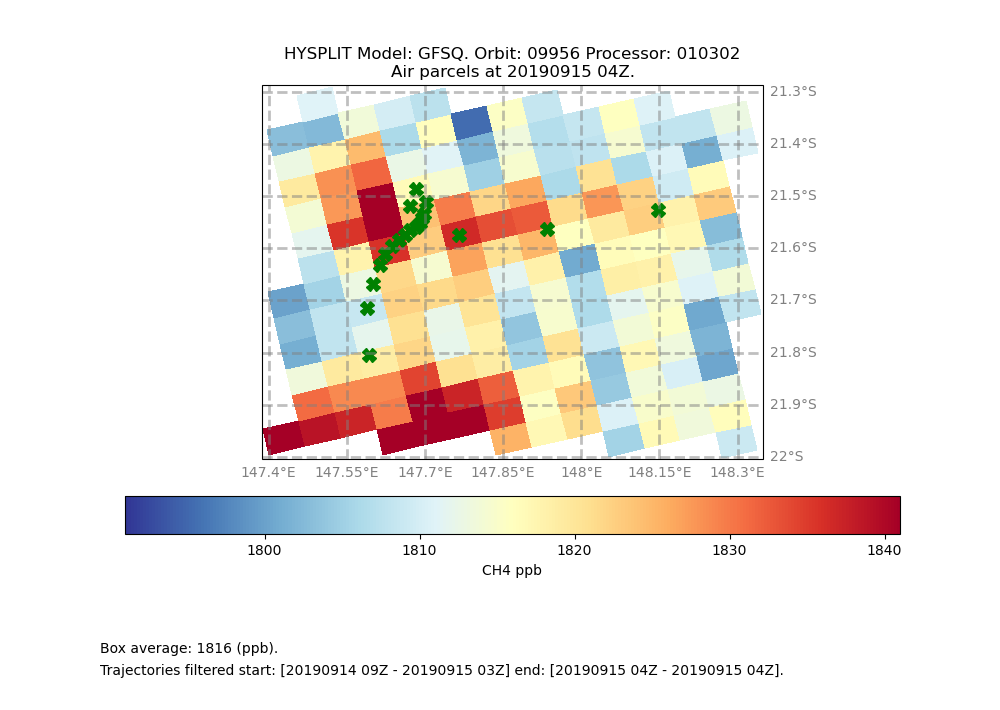
The endpoints of these trajectories, representing the plume centre at the TROPOMI overpass time, are shown as green crosses in Figure 28. Two distinct groups emerge. The first comprises five endpoints located west of 145°E, corresponding to puffs released between 2019-09-14 04Z and 08Z (around sunset). The second group lies close to the Hail Creek mine and includes hourly trajectories for puffs released from 2019-09-14 09Z (approximately 7p.m. local time) through 2019-09-15 03Z, one hour before the TROPOMI observation.

To examine this further, the second group trajectories are plotted in Figure 29. Emissions released over the full 18-hour period remain within the TROPOMI image domain, reflecting the light and variable winds typical of the nocturnal stable boundary layer, consistent with both Moranbah AWS observations and the TROPOMI imagery. Although the simulated trajectories are displaced slightly south of the plume seen in TROPOMI, the agreement is reasonable, particularly in the location of the maximum enhancement, which the TROPOMI image places near 147.6°E, 21.55°S.

Another notable feature is that puffs released between 2019-09-14 09Z and 2019-09-15 00Z remained near the mine throughout the night before being advected during the transition to the Convective Mixed Layer (CML) . They converge into a narrow cluster of endpoints along 147.6°E, coinciding with the area of elevated ${\mathrm{CH}}_4$ enhancement. This indicates that the plume is highly inhomogeneous, with its leading edge containing emissions accumulated over roughly 14 hours. This behaviour supports our conclusion that non-steady flow conditions significantly affect the performance of the CSF and IME algorithms.

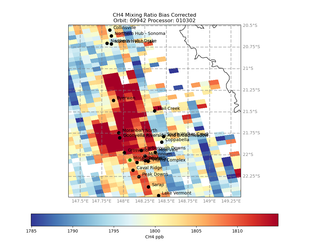
HYSPLIT can also be used to compute backward trajectories, allowing us to estimate the background concentration associated with air masses contributing to the observed plume. Specifically, if emissions occurred at 2019-09-15 00Z, a 20-hour backward trajectory can be used to identify the location of that air parcel at the time of the previous TROPOMI overpass (2019-09-14 04Z). For the orbit under study (09956), the corresponding earlier overpass is orbit 09942, shown in Figure 30.

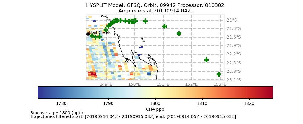
This approach is inherently imprecise, as the background air mass may change its ${\mathrm{CH}}_4$ concentration before reaching the mine due to turbulent diffusion and contributions from other emission sources encountered along the way. The locations of the backward trajectory puffs at the time of orbit 09942—corresponding to air parcels passing over Hail Creek between 2019-09-14 05Z and 2019-09-15 03Z—are shown in Figure 31.

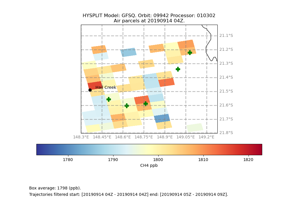
By zooming in, we can estimate background values for the backward trajectory puffs that reached Hail Creek between 2019-09-14 05Z and 09Z, that is, before the likely onset of SNBL conditions. Under a pure advection assumption, these background concentrations range from approximately 1800 ($\mathrm{ppb}$) to 1810 ($\mathrm{ppb}$) (see Figure 32). However, background values relevant to emissions released after sunset cannot be determined, as the corresponding air parcels originate over the ocean at the time of the preceding TROPOMI overpass (orbit 09942).

In summary, the HYSPLIT forward modelling shows a clear discontinuity in plume behaviour at approximately 7 p.m. local time (sunset) and again near 7 a.m. (sunrise). This agrees well with the Moranbah AWS observations, unsurprising given that these observations are likely assimilated into the GFSQ dataset used by HYSPLIT . The substantial changes in wind conditions across these transitions violate the steady flow assumption required by the CSF algorithm.

The use of backward trajectories to estimate background concentrations illustrates both the potential of this approach and its inherent complexities. Background values inferred from the previous day may be substantially altered before reaching the source region, not only through turbulent diffusion but also through the incorporation of emissions from other upwind sources. As a result, background estimates derived in this manner must be interpreted with considerable caution.

Finally, it is important to consider the applicability of HYSPLIT modelling in this case. As noted earlier, HYSPLIT has significant limitations. In particular, the modelled overnight trajectories likely do not capture the accumulation of emissions within the mine pit, as such fine scale features fall well below the resolution of the GFSQ dataset. Nevertheless, the reasonable agreement between the model output and the TROPOMI observations is encouraging. A similar concentration pattern might have been reproduced if the model were capable of representing local overnight flow conditions.

CSF

The first consideration is the applicability of this method. It relies on the assumption that the mass within the box remains constant over the time required for the plume to pass through it. Because the algorithm averages across up to 12 individual box models, the validity of this assumption may differ for each one.

Analysis of the MSLP charts, Moranbah AWS observations, and HYSPLIT modelling indicates that an SNBL developed during the night, resulting in non-uniform plume flow. This suggests that the CSF method is not applicable for transects near the plume head, though it may still be applicable for transects closer to the source. Because this dataset was used in Sadavarte, et al., 2021 , we review the CSF results here and compare them with those from the TM and IME methods.

We use the TROPOMI file processed with version 010302, as version 020400 was released after the publication of the original study.

The key elements of the CSF modelling for this case are summarised in the three figures previously introduced during the description of the CSF algorithm (Figures 8, 9 , and 10 in TROPOMI CSF Software ). Figure 8 shows the downwind box, upwind box, transects, and all valid pixels. This figure demonstrates strong pixel coverage within the downwind box, making this orbit a suitable sample for detailed analysis.

The CSF identified positive pixels (i.e., those classified as part of the plume) are shown in Figure 9 . The pressure averaged BLH wind speed is 5.8 ($\frac{m}{s}$), satisfying the validity criterion. The algorithm computed a background value of 1812.372 ($\mathrm{ppb}$) as the mean of the 31 pixels in the upwind box. It reported a successful retrieval for this orbit, yielding an emission rate of 32.256 ($\frac{t}{\mathrm{hour}}$), corresponding to an annualised value of 282.563 ($\frac{\mathrm{Gg}}{\mathrm{year}}$).

The third and final chart, Figure 10 , shows the emission rates calculated for each transect. It presents the emission estimates derived from the individual box model surfaces. Transects 4-14 are considered valid, while transect 15 is rejected because it does not intersect the plume. Transects 8-13 exhibit substantially higher emission rates. Since the transects represent sequential cross-sections through which the plume passes, differences of this magnitude indicate that the flow is not in steady state. This behaviour is likely due either to variable emission rates or, more plausibly, to changes in meteorological conditions associated with the presence of the SNBL.

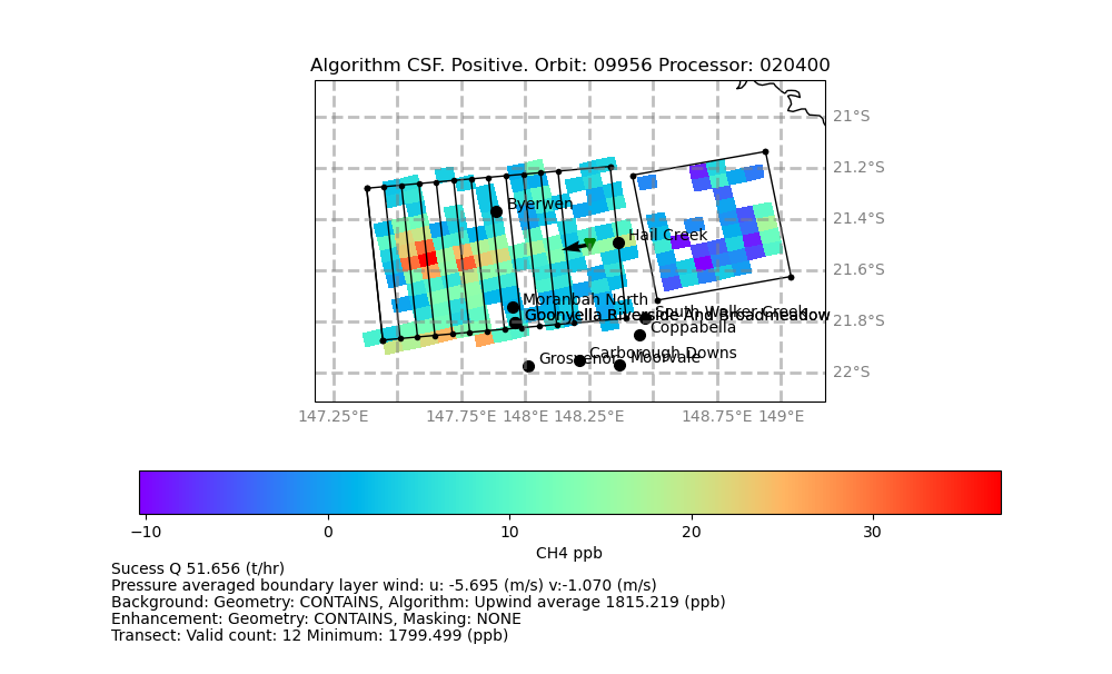
It is informative to compare these results with those obtained using the CSF method applied to the TROPOMI image processed with algorithm 020400 (see Figure 33). In this version, the plume is identified as significantly wider, and the corresponding emission estimate increases from 32.256 ($\frac{t}{\mathrm{hour}}$) to 51.656 ($\frac{t}{\mathrm{hour}}$). This highlights the sensitivity of the method to both the TROPOMI processing algorithm and the determination of key elements such as plume extent, transect placement, and background selection.

TM

The first consideration is whether this method is applicable. In the absence of more detailed information, we adopt the plume shape and background determined by the CSF model and use transect 15. Analysis of the MSLP fields, Moranbah AWS observations, and HYSPLIT modelling indicates that an SNBL developed during the night, producing a finite plume contained within the selected box and exhibiting no flow through its boundaries. Under these conditions, the TM approach may be appropriate for this box. However, if the plume boundaries were defined instead using transects 4-14, the method would not be valid, as non-zero flow would occur across the box boundary (see Table 14).

The starting point for this method is shown in Figure 9. It can be argued that some of the included pixels are artefacts of the background-estimation process and should be excluded from the calculation. In addition, we have no estimate of IME(0) (the mass contained within the plume at the onset of SNBL) so we assume it to be zero. Both of these simplifications will bias the TM results upward, leading to an overestimation of the emission rate.

Calculating the pixel area included in the plume requires the same type of geometric decision used in the CSF algorithm. In this implementation, we adopt the INTERSECTS geometry, computing each pixel's contribution as the area of its intersection with the plume. This is the most conservative choice and results in the largest estimated emission rate.

The last parameter used by TM is time of plume generation. Here we use results of HYSPLIT modelling using trajectories for puffs emitted hourly for 24 hours before the image time. HYSPLIT modelling estimates that 18 of these puffs were within downwind box at the time of the image (T=18).

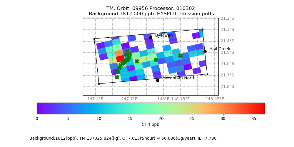
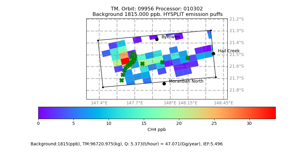
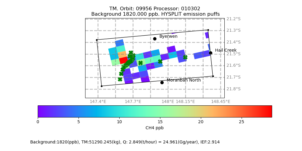
Below, we illustrate the plume shape and the pixels included under three different background values 1812, 1815, and 1820 ($\mathrm{ppb}$) (see Figures 34, 35 and 36). We leave it to the reader to determine the most appropriate plume extent and background value.

The emission rates for the range of background choices, along with their comparison to the CSF outputs, are presented in Table 20 below.

In the absence of more detailed information, using a background value of 1812.373 ($\mathrm{ppb}$), estimated as the upwind box average following Sadavarte, et al., 2021 , and summing the excess mass over the plume area yields an estimated plume mass of approximately 147.329 ($t$) of ${\mathrm{CH}}_4$. This corresponds to an annualised emission of 71.701 ($\frac{\mathrm{Gg}}{\mathrm{year}}$) and an implied emission factor IEF of 7.017 ($\frac{g}{\mathrm{kg}}$) when using Queensland Government activity data.

Because the algorithm is highly sensitive to the selected background value and plume definition, determining the actual emission rate is challenging and likely requires expert judgement. However, based on the table above, one can infer that under SNBL conditions, the CSF derived estimates are approximately three to five times higher than those obtained using the TM method.

IME

Once again, the first issue to consider is whether this method is valid. IME is a special case of the TM approach, relying on the assumption that residence time can be expressed as the box length divided by the wind speed. This requires two conditions to hold:

1. no flow through the lateral boundaries, and
2. a constant wind speed throughout the box.

Using the box associated with transect 15 satisfies the first assumption (no lateral flow) but violates the second (constant wind). Conversely, using the box defined by transects 4-8 satisfies the constant wind assumption but violates the noflow condition. Transects 9-14 appear to violate both assumptions.

To illustrate this, and again using the CSF output shown in Figure 9 as a starting point, we constructed 11 models based on the boxes defined by each transect and the downwind box boundary that intersects the source. The key elements of these calculations are summarised in Table 21. For transects 4-8, the model output oscillates between 11 and 17 ($\frac{t}{\mathrm{hour}}$) before increasing to 29.764 ($\frac{t}{\mathrm{hour}}$) by transect 13.

Summary

This case study demonstrates the following:

• A stable nocturnal boundary layer SNBL formed during the night of 14-15 September 2019, as indicated by the MSLP analysis and Moranbah AWS observations.
• The plume exhibits a non-uniform concentration distribution, as shown by the HYSPLIT modelling results.
• The non-uniform wind field limits the applicability of the CSF algorithm.
• CSF outputs vary substantially depending on the TROPOMI processor version. Using processor 010302, the algorithm identifies a plausible downwind box that captures the Hail Creek plume; using processor 020400, the algorithm identifies a much wider box that likely includes contributions from Bowen Basin mines.
• In this case, the TM algorithm appears to be the most appropriate approach and produces emission estimates approximately three to five times lower than those from the CSF method when using the same background concentration.
• The non-uniform wind field also limits the applicability of the IME algorithm.