Computational stability

In this section, we examine the impact of specific algorithmic choices on the resulting calculations. As before, we use TROPOMI orbit 09956 processor 010302 for this analysis.

The algorithm description does not clarify how pixels are associated with the domain. While this may appear to be a minor technical detail, it has meaningful practical implications. The chosen method directly affects the calculation of both the background concentration and the downwind box — parameters to which the algorithm is highly sensitive.

To illustrate this issue, both the domain and each pixel can be treated as polygons. Under this framework, two interpretations of their relationship are possible: containment and intersection. A pixel can be considered part of the domain either when its polygon lies entirely within the domain, or when its polygon merely intersects the domain boundary. In the remainder of this report, these relationships are referred to as “CONTAINS” and “INTERSECTS”, respectively.

Another possible interpretation is to treat each pixel as a point defined by its centre. Under this approach, a pixel is considered within the domain if its centre lies inside the domain boundary. In the remainder of this report, this geometrical relationship is referred to as “CENTER”.

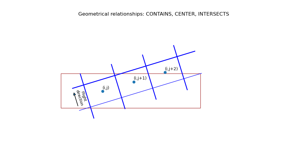
As illustrated in Figure 20 , the choice of geometrical relationship affects which pixels are included in the domain. Under INTERSECTS, all three pixels are included; under CENTER, only pixels (j,i) and (j,i+1) are included; and under CONTAINS, only pixel (j,i) falls within the domain. Physically, this means that using CENTER instead of CONTAINS effectively adds about half a pixel, and using INTERSECTS can add up to another half, depending on geometry. The exact magnitude of this change depends on pixel size, which varies with the viewing zenith angle. From mathematical perspective, these relationships are ordered: if CONTAINS is true, then CENTER is also true; and if CENTER is true, then INTERSECTS is necessarily true.

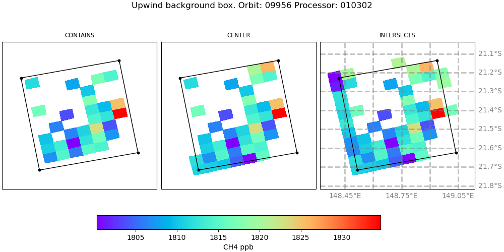
The impact of the chosen geometrical relationship on the background box pixel selection is illustrated in Figure 21 , and the resulting background values are summarised in Table 14. All calculated values satisfy the validity criterion of having more than 20 contributing pixels.

In the absence of independently measured background values, several approaches can be used to estimate the background. Common methods include:

• The average over a 0.5° x 0.5° box located 0.5° upwind of the source Sadavarte, et al., 2021
• The average over a 0.5° x 0.5° box directly upwind of the source Schneising, et al., 2023
• The domain median Sadavarte, et al., 2021
• A data-driven quantile method, where the selected quantile is constrained such that the difference between it and the first decile is less than twice the measurement precision of the LGR UGGA ${\mathrm{CH}}_4$ analyser $(2\times ~\mathrm{1.4}ppb)$ for ${\mathrm{CH}}_4$. See lines 221 - 241 of supplementary notes to Borchardt, et al., 2025 .
• Proprietary background-estimation approaches (e.g. Kayrros , GHGSAT ).

In the supplementary notes of Sadavarte, et al., 2021 Supporting Information , the authors state that both the domain median and the upwind-box average were evaluated as background-estimation methods.

All of the background-estimation methods described above are statistical in nature and reflect the absence of direct background measurements. However, the choice of background value critically influences both the determination of the downwind-box enhancement and the transect-level enhancement, making it one of the most sensitive parameters in plume-detection algorithms. To illustrate the non-linear consequences of selecting a particular background value, we consider a continuous synthetic mixing ratio profile representing the cross-plume signal along a transect, as defined in Equation 16 .

To approximate TROPOMI measurements across ten pixels, we use the integral of this synthetic mixing ratio function (see Equation 17), which can be evaluated analytically. Each of the ten integrals—computed over successive unit intervals (e.g., 0.5-1.5, 1.5-2.5, etc.) — represents the mixing ratio measured within a single pixel.

In addition, we consider three different background values: 1841, 1839.5 and 1838 ($\mathrm{ppb}$). All of these elements are shown in Figure 22 below.

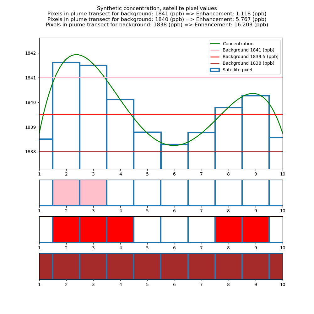
From this figure, we observe that with a background value of 1841.0 ($\mathrm{ppb}$), only pixels 2 and 3 exhibit positive enhancement. With a background of 1839.5 ($\mathrm{ppb}$), pixels 2, 3, 4, 8, and 9 contribute to the enhancement. When the background is set to 1838 ($\mathrm{ppb}$), all pixels from 1 to 10 show enhancement. This illustrates the strong non-linear dependence of the enhancement field on the chosen background value.

In this example, any further decrease of the background value below 1838 ($\mathrm{ppb}$) (the minimum value in the transect) would add a fixed increment of 10 to the total enhancement—corresponding to 10 pixels each gaining 1 unit of enhancement for every unit decrease in the background.

This example demonstrates that the choice of background value directly influences both the inferred plume shape and the resulting enhancement calculations.

In practice, this issue is further complicated by missing values (e.g., due to cloud cover). This requires maintaining a clear distinction between missing values—where no enhancement can be estimated—and valid measurements that fall below the background value, for which the enhancement should be set to zero while the pixel remains classified as valid.

The rotations selected by the algorithm under the different strategies are summarised in Table 15 and range from -10° to +15°, depending on the chosen configuration.

The model downwind box lengths selected by the algorithm for the different geometrical relationships are listed in Table 16 and range from 77 ($\mathrm{km}$) to 99 ($\mathrm{km}$), depending on the configuration.

The model downwind box widths selected by the algorithm for the different strategies are listed in Table 17 and range from 22 ($\mathrm{km}$) to 66 ($\mathrm{km}$), depending on the configuration.

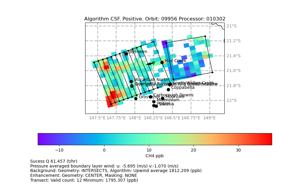
Finally, we calculated emission rates for all 18 combinations of geometrical relationships and masking strategies. The results, summarised in Table 18, range from 20.03 ($\frac{t}{\mathrm{hour}}$) to 61.457 ($\frac{t}{\mathrm{hour}}$). All runs use identical input datasets and differ only in the geometrical and masking treatments applied to the pixels.

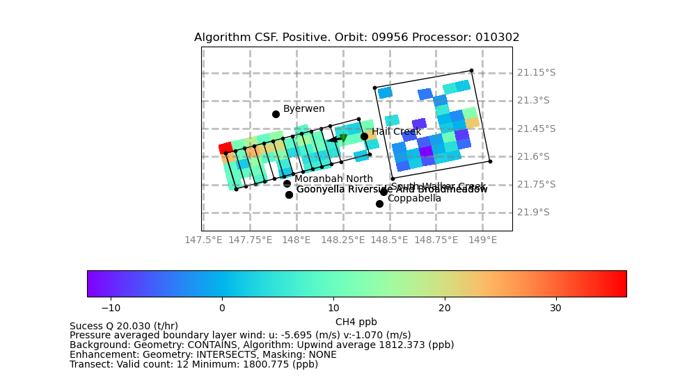
The default case is shown in Figure 12 , while the differences between the two most extreme configurations are illustrated in Figure 23 and Figure 24 below.

It is difficult to establish what constitutes acceptable algorithmic stability. In the examples above, we introduced small perturbations in how pixels are classified. Changing the geometry from CONTAINS to CENTER, and from CENTER to INTERSECTS, effectively expands the domain by at most half the pixel diagonal (approximately 4.5 ($\mathrm{km}$) for a 5.5 x 7 ($\mathrm{km}$) pixel). Yet these small geometric adjustments can produce variations of emission estimate up to 100%. Use of destriped imagery may help reduce this sensitivity, as it would likely decrease variability between neighbouring pixels.